Extend your BrainVision Analyzer 2 to its full potential with Solutions
by Dr. Bastian Schledde
Scientific Consultant (Brain Products)
 Are you looking for extensions for BrainVision Analyzer 2? They are called Solutions! Scientists from various fields of research use them to tweak Analyzer to their needs. Analysis of non-EEG sensor data, sleep data, single trials and time-frequency domain exports are only some examples where users can benefit from our solutions.
In the following we present our most popular solutions and show how they add valuable functionality to Analyzer 2. We will start with general remarks and installation instructions and continue with some selected use-cases dedicated to specific analysis needs. At the end we present generally useful solutions that many of our users can profit from.
General remarks and installation instructions
BrainVision Analyzer 2 is appreciated for its easy-to-use yet powerful signal processing ability. Analysis pipelines created from the rich collection of Transformations cover most analysis needs while being extremely memory efficient. As scientific methodology is rapidly evolving, occasionally researchers will miss a function or method that is not implemented as a transformation. At Brain Products Scientific Support, we offer a variety of extensions to Analyzer 2 that fill in this gap. We call them Solutions. They are usually created in first response to a frequently needed functionality and over time, we have grown a significant library of them. Solutions are free of charge for any Analyzer 2 user. Once they are installed you can use them almost as any other transformation.
Most popular solutions can be directly downloaded from our website. You have the option to download all of them at once or only individual ones. Either way you only need to run the installer and open Analyzer 2 to have them in your Solutions ribbon menu (see below).

If Analyzer 2 was already open, click Solutions > Help > Refresh Solutions to see them. Under the Solutions Help menu you will find the documentation for each of them. If you are struggling with a certain task in Analyzer 2, our Scientific Support is always happy to help. We might send you a solution that is not available on our website, in this case you receive a solutions file (*.vaso), that you need to add to a subfolder of the Solutions directory on your Analyzer 2 installation path. The default path is: C:\Vision\Analyzer2\Solutions.
One word on macros – yes, solutions are basically compiled macros. You can add your own functions to Analyzer 2 by writing a Sax Basic macro and running it through the Macro ribbon menu. This topic will not be covered in this article. You can find more information on it on our website.
Solutions to help with specific analyses
Sensor Data
If you are working with signals from non-EEG sensors, we offer a range of solutions that you might find useful. For instance, you can analyze acceleration data, ECG profiles, EMG or GSR Peaks, Pulse transit times and width with the help of solutions. We have recently described how you can do that in our Support Tip “Offline analysis of sensor data in BrainVision Analyzer”.
Sleep
If you are a sleep researcher, you might be interested to know how to score and use sleep stages in Analyzer 2. Our Sleep Scoring solution allows you to manually score your data or inspect and edit imported sleep scores. For this purpose, we introduced the SleepStage marker dedicated to sleep research. Its description indicates the type of physiological state i.e., sleep stage N1, N2, N3, N4, REM, or Wake or the absence of a score (None). The Sleep Scoring solution recognizes these markers and allows you to edit them.
You can navigate the sleep data in steps of the desired scoring interval (typically 30 seconds). The frequency-spectra or topography can be displayed simultaneously to support the scorer. A full night hypnogram displaying all scores can be opened in a Microsoft Excel® sheet. Once scoring is finished, a Sleep Report can be generated. It summarizes important sleep parameters such as sleep latency, sleep efficiency, duration of stages and composition of sleep cycles. The approved scores remain as markers in the dataset and can be used for Segmentation in a sleep-informed analysis in Analyzer 2. This solution will be available from our website from November 2021.
If you are interested in a demonstration of the solution, feel free to watch the recording of our webinar about “Sleep Research and Sleep Scoring Solution”.
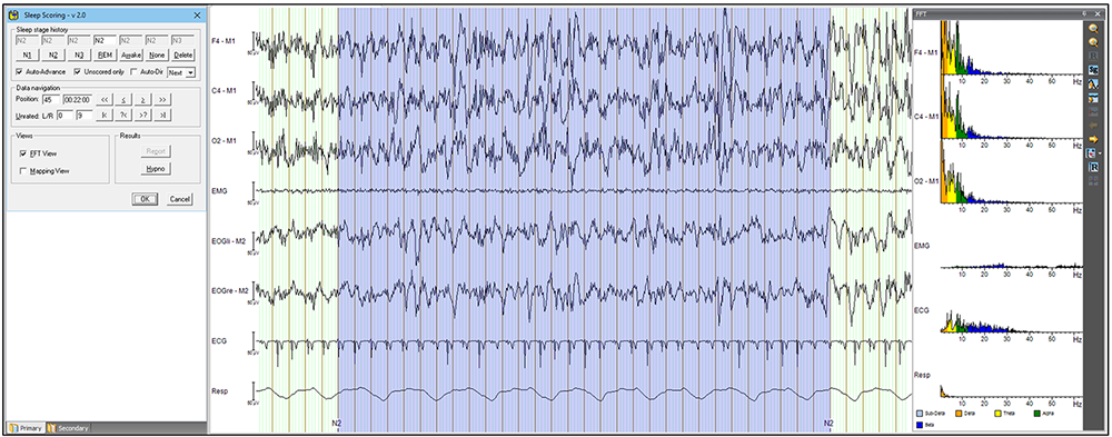
Figure 1 Sleep Scoring in Analyzer 2 with the display of the frequency data of the current scoring interval.
Single trial analysis
Analyzer 2 was originally designed for ERP analysis. Many ERP studies need to extract features of ERP components only after performing an Average across trials. Analyzer’s transformations and exports are designed for this approach and offer feature extraction from averaged data. Solutions add the possibility to also perform single trial analysis.
The Peak Detection transformation for example, detects peaks on averaged data and the MinMax Marker solution on a single trial level. It allows you to place Peak markers at the maximum and/or minimum in a certain interval of each segment.
Likewise, where Area Information and Peak Information Export modules work on averaged datasets, you can export data from single trials with the solutions described in the section Solutions for exports below. There are solutions for time, frequency, or time-frequency domain exports.
Before the detection and export of peaks, it often makes sense to assess the ERP on a single trial level. For example, to estimate the variability of components across segments or to visually inspect a set of trials at once. You can do this with the Stacked Plot solution. It will display all segments stacked on top of each other (see Figure 2). The solution is using the time-frequency view in Analyzer 2 to display trial number on the ordinate and time on the abscissa. Amplitude is shown on a color scale that can be configured through the view settings.
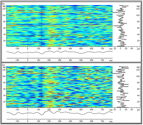
Figure 2. Stacked Plot view: the solution utilizes the time-frequency view in Analyzer 2 to show multiple stacked trials. For this reason, the label of the ordinate is showing Hz instead of trial number.
Solutions for exports
Our most popular solutions are exports. These provide exports of time, frequency or time-frequency domain data from averaged or single-trial history nodes. For a detailed overview about exports please read our Support Tip “Exports for all occasions – A selective overview of Analyzer 2’s most useful export options”.
Peak Export: Despite its name the solution exports not only various peak measures such as amplitude, latency, peak-to-peak distance and the area under the curve but also average amplitudes within a time interval. This is the go-to solution if you need to export single trial, time domain data.
FFT Band Export: Like the Peak Export this solution can be used to export single-trial data from a selected frequency range. It allows you to export individual values as well as many aggregation options such as area under curve measures, average or the raw sum.
Wavelet Data Export: If you are using Wavelets to decompose your data into the time-frequency domain this solution is essential. You can specify a time and frequency range (see Figure 3) and then export the sum or average of this area to a text file. It is applicable for both real (e.g. power) or complex values. It is now also possible to export into a file with comma separated values (*.csv), making the transfer to other software even easier.
Create MAT File: Complementary to the Matlab transformation, that interfaces directly with the application, this solution allows you to create a MATLAB® compatible file (*.mat) with the data of the current history node. For each channel a separate variable is created. Note that time-frequency domain data cannot be exported with this solution.
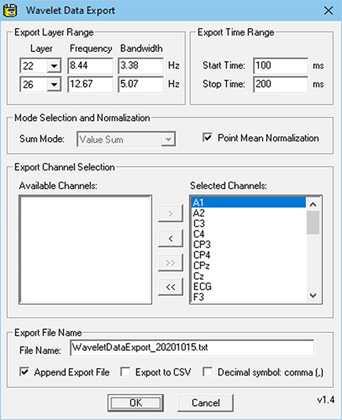
Figure 3. Interface of the Wavelet Data Export solution.
Solutions for parameter extraction
The Write Markers solution has found many useful applications despite its simplicity. It collects basic information of selected markers and writes them to an external text file. Marker information includes Description, Type, Position, Duration and Amplitude at the marker position. An example file is shown in Figure 4. It is generated from a continuous dataset and only includes selected output information. If the dataset is segmented, each row in the file corresponds to a segment. If it is continuous, you can specify a marker that will trigger a new line or row. In this example the “S_20” marker was used. In the exported file, the position of this marker is reset to zero.
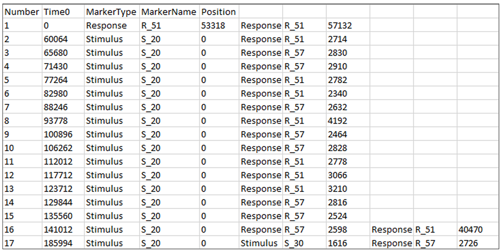
Figure 4. Example output of the Write Markers solution.
The position of all other markers in the same row is exported as the distance to the previous “S_20” marker. This feature allows you to inspect marker placement and to plan a marker-based segmentation before actually implementing it.
This export is also quite useful to extract:
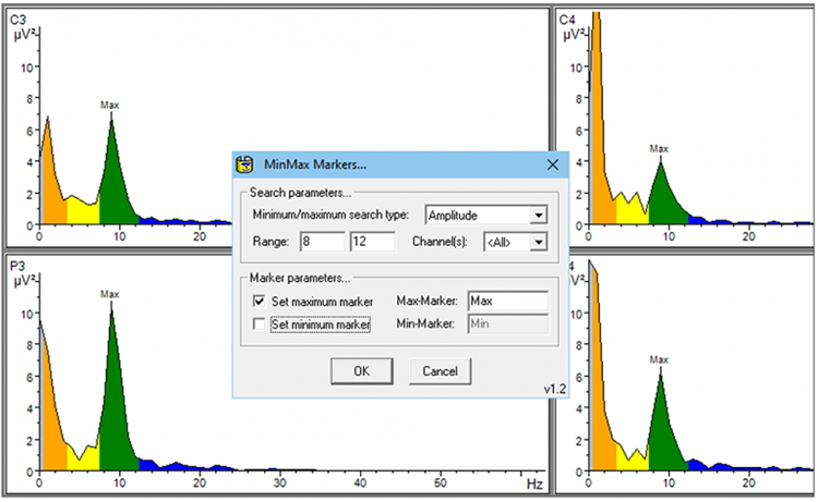
Figure 5. Example of the MinMax Marker solution applied to FFT (frequency domain) data to identify peak frequencies.
Other popular solutions
Recode Markers: If you are interested to explore the relationship between the behavioral response and the EEG, this solution might be worth noticing. It allows you to select a group of segments based on the temporal distance between markers. Typically, the distance between a Stimulus and Response marker is used to reflect the reaction time. Available groupings are Median/Mean Split, Mean ± SD, Upper/Lower percentages, Middle fraction and more. It is also possible to define your own fractions in percentage or time range. The inserted marker (Type “Comment”) can be used within Segmentation to create a group ERP. Additionally, statistics such as the Mean, Median and Standard Deviation (SD) of the marker distances (e.g. reaction time) are reported in the Operation Infos of the Marker Recode history node.
Set Markers: Have you ever been in need to add a marker to your dataset? Maybe because you realized only after recording that it is needed or because it was simply forgotten. Of course, you can add or edit markers with Edit Markers transformation, but if you need to place a marker in a fixed distance to another existing marker this solution will help. It allows you to insert markers with a fixed or randomized temporal distance to all markers of a selected Type and Description. This solution will be available from our website from November 2021.
Read Coordinates: If your dataset is lacking electrode coordinates but they are available in an external file, you can load it with this solution. You can specify the type of coordinates used (cartesian or spherical) and instruct the solution where to find the information in the file. This makes it possible to read from any electrode coordinate file if it is in a compatible text form. The solution also converts coordinates. In Analyzer 2 only spherical coordinates are used and if yours are specified in cartesian it will convert them. This solution will be available from our website from November 2021.
Moving Average: Some analyses require to estimate the envelope of the signal, for example in EMG analysis. The Moving Average solution can be used to smooth the data, similar to a low-pass filter. Each value is replaced with the average of a time-window centered on the current data point. It offers some extra options such as rectification before or subtraction instead of replacing with the average.
Concluding remarks
To grasp the full processing power and skill of Analyzer 2 it is good to know Solutions and the range of functionality that they add to it. This article provides a glimpse of the full spectrum that is available with the solutions that are useful for most researchers. If you are stuck with your analysis and need to advance your pipeline beyond what you can do with transformations our tip is: browse through our solutions and find out whether they can help you. If you don’t find anything that fits your pipeline, contact us, we have more! Please get in touch with us via support@brainproducts.com and we will do our best to find a solution for you.

